Prepare and load your own data

This page shows you how to format and load your own custom data into your local instance. This is step 2 of the recommended workflow.

• Overview
  • Files and directory structure
• Prerequisite steps
  • Step 0.1: Determine whether you need new entities or entity types
    • Entities and entity types
    • Search for an existing entity / entity type
  • Step 0.2: Identify your statistical variables
  • Step 0.3: Choose between “implicit” and “explicit” schema definitions
    • Variable schemas
• Prepare your data using implicit schema
  • Step 1: Provide variables and observations in CSV
  • Step 2: Write the JSON config file
• Prepare your data using explicit schema
  • Step 1: Define statistical variables in MCF
    • (Optional) Define a statistical variable group
  • Step 2: Prepare the CSV observation files
  • Step 3: Write the JSON config file
• Load local custom data
  • Configure environment variables
  • Start the Docker containers with local custom data
  • Verify your data
  • Inspect the SQLite database

Overview

Custom Data Commons requires that you provide your data in a specific schema, format, and file structure. We strongly recommend that, before proceeding, you familiarize yourself with the basics of the Data Commons data model by reading through Key concepts, in particular, entities, statistical variables, and observations.

At a high level, you need to provide the following:

• All observations data must be in CSV format, using the schema described later.
• You must also provide a JSON configuration file, named config.json, that specifies how to map and resolve the CSV contents to the Data Commons schema knowledge graph. The contents of the JSON file are described below.
• Depending on how you define your statistical variables (metrics), you may need to provide MCF (Meta Content Framework) files.
• If you need to define new custom entities, please see Define custom entities for details.

Files and directory structure

You can have as many CSV and MCF files as you like, and they can be in multiple subdirectories (with an additional configuration option). There must only be one JSON config file, in the top-level input directory. For example:

my_data/
├── config.json
├── (nodes1.mcf)
├── datafile1.csv
├── datafile2.csv
└── some_more_data/
    ├── (nodes2.mcf)
    ├── datafile3.csv
    └── datafile4.csv

The following sections walk you through the process of setting up your data.

Prerequisite steps

The following sections describe the high-level conceptual work you need to do before starting to write your data and config files.

Step 0.1: Determine whether you need new entities or entity types

Data Commons is optimized to support aggregations of data at geographical levels, such as city, state, country, and so on. If your data is aggregated by place, these are supported as entities out of the box. If, however, you want to aggregate data for entities that are not places, then you may need to define new entities, and possibly even entity types.

In addition, even if you aggregate by geographical area, you may want to measure things (known as a “population type” in the graph) that are not already in the graph. In that case, you might want to to define a new entity type, so that you can join with other data sets that measure the same thing. For example, let’s say you have a metric that counts the number of beds in hospitals. The existence of the Bed entity type allows you to join your data with other sources with a similar metric.

Entities and entity types

Schema.org and the base Data Commons knowledge graph define entity types for just about everything in the world. An entity type is a high-level concept, and is derived directly from a Class type. The most common entity types in Data Commons are place types, such as City, Country, AdministrativeArea1, etc. Examples of other entity types are Hospital, PublicSchool, Company, BusStation, Campground, Library etc. It is rare that you would need to create a new entity type, unless you are working in a highly specialized domain.

An entity is an instance of an entity type. For example, for PublicSchool, base Data Commons has many U.S. schools in its knowledge graph, such as nces/010162001665 (Adams Elementary School) or nces/010039000201 (Wylam Elementary School). Base Data Commons contains thousands of places and other entities, but it’s possible that it does not have specific entities that you need. For example, it has about 100 instances of Company, but you may want data for other companies besides those. As another example, let’s say your organization wants to collect (possibly private) data about different divisions or departments of your org; in this case you would need to define entities for them.

Note: You should always reuse existing entity types and entities from base Data Commons rather than re-defining them. This way, you get all the properties already defined for those entities and all their linked nodes, and can more easily join with base data if needed.

Search for an existing entity / entity type

Unfortunately, it is currently not possible to get a full list of entity types or entities in the Data Commons UI. To do a complete search for an entity type or entity, you need to use the REST or Python APIs.

To search using the REST APIs:

1. Use the Node API through your browser to get a complete list of entity types: see Get a list of all existing entity types in the REST API V2 reference. Be sure to set the nextToken parameter until you find the relevant entity type or no nextToken is returned in the response. If you don’t find an entity type that matches your needs (very rare), you will need to create one.
2. If you find a relevant entity type, note the DCID of the entity type of interest. The DCID of entity types is usually a meaningful name, capitalized, such as Hospital or PowerPlant or PublicSchool.

3. Use the Node API through your browser to look up all incoming arcs by the typeof property:

   https://api.datacommons.org/v2/node?key=AIzaSyCTI4Xz-UW_G2Q2RfknhcfdAnTHq5X5XuI&nodes=ENTITY_TYPE&property=<-typeOf

   ENTITY_TYPE is the DCID you’ve obtained in the previous step, such as Hospital or PublicSchool. For example:

    https://api.datacommons.org/v2/node?key=AIzaSyCTI4Xz-UW_G2Q2RfknhcfdAnTHq5X5XuI&nodes=PublicSchool&property=<-typeOf
   

4. If your entity is listed, note its DCID. If you are unable to find a relevant entity, you will need to create one. See Work with custom entities for complete information.

To search using the Python APIs:

1. Start your Python interactive environment and create a client for the base Data Commons.
2. Call the Node method fetch_all_classes: see Get node properties for details. (Tip: Use the to_dict() method on the response to get readable output.) If you don’t find an entity type that matches your needs (very rare), you will need to create one.
3. If you find a relevant entity type, note the DCID of the entity type of interest. The DCID of entity types is usually a meaningful name, capitalized, such as Hospital or PowerPlant or PublicSchool.

4. Use the fetch_property_values method to find all the instances of the type:

   client.node.fetch_property_values(node_dcids="ENTITY_TYPE", properties="typeOf", out=False)

   ENTITY_TYPE is the DCID you’ve obtained in the previous step. For example:

    client.node.fetch_property_values(node_dcids="PublicSchool", properties="typeOf", out=False)
   

5. If your entity is listed, note its DCID. If you are unable to find a relevant entity, you will need to create one. See Work with custom entities for complete information.

Step 0.2: Identify your statistical variables

Your data undoubtedly contains metrics and observed values. In Data Commons, the metrics themselves are known as statistical variables, and the time series data, or values over time, are known as observations. While observations are always numeric, statistical variables must be defined as nodes in the Data Commons knowledge graph.

Statistical variables must follow a certain model: it includes a measure (e.g. “median age”) on a set of things of a certain type (e.g. “persons”) that satisfy some set of constraints (e.g. “gender is female”). To explain what this means, consider the following example. Let’s say your dataset contains the number of schools in U.S. cities, broken down by level (elementary, middle, secondary) and type (private, public), reported for each year (numbers are not real, but are just made up for the sake of example):

The measure here is a simple count; the set of things is “schools”; and the constraints are the type and levels of the schools, namely “public”, “private”, “elementary”, “middle” and “secondary”. All of these things must be encoded as separate variables. Therefore, although the properties of school type and school level may already be defined in the Data Commons knowledge graph (or you may need to define them), they cannot be present as columns in the CSV files that you store in Data Commons. Instead, you must create separate “count” variables to represent each case. In our example, you would actually need 6 different variables:

• Count_School_Public_Elementary
• Count_School_Public_Middle
• Count_School_Public_Secondary
• Count_School_Private_Elementary
• Count_School_Private_Middle
• Count_School_Private_Secondary

If you wanted totals or subtotals of combinations, you would need to create additional variables for these as well.

Step 0.3: Choose between “implicit” and “explicit” schema definitions

Custom Data Commons supports two ways of importing your data:

• Implicit schema definition. This method is simplest, and does not require that you write MCF files, but it is more constraining on the structure of your data. You don’t need to provide variables and entities in DCID format (although you may); but you must follow a strict column ordering, and variables must be in variable-per-column format, described below. Naming conventions are loose, and the Data Commons importer will generate DCIDs for your variables and observations based on a predictable column order or for entities based on the column you identify. This method is simpler and recommended for most datasets.

• Explicit schema definition. This method is a bit more involved, as you must explicitly define DCIDs for all your variables (and entity types if needed) as nodes in MCF files. All variables in the CSVs must reference DCIDs. Using this method allows you to specify variables in variable-per-row format and to specify additional properties of variables or entities, offering greater flexibility. There are a few cases for which this option might be a better choice:

  • You have hundreds of variables, which may be unmanageable as separate columns or files.
  • You want to be able to specify additional properties, for example, unit of measurement, of the observations at a more granular level than per-file. As an example, let’s say you have a variable that measures financial expenses, across multiple countries; you may want to be able to specify the country-specific currency of each observation.
  • In the case that you are missing observations for specific entities (e.g. places) or time periods for specific variables, and you don’t want to have lots of null values in columns (sparse tables).

Variable schemas

To illustrate the difference between variable-per-column and variable-per-row schemas, let’s use the schools example data again. In variable-per-column, you would represent the dataset as follows:

Variable-per-column schema

The names that appear in the columns and rows don’t need to be DCIDs or follow any convention, because the columns must always be specified in this exact sequence:

ENTITY, OBSERVATION_DATE, STATISTICAL_VARIABLE1, STATISTICAL_VARIABLE2, …

In variable-per-row, the same dataset would be provided as follows:

Variable-per-row schema

The names and order of the columns aren’t important, as you can map them to the expected columns in the JSON file. However, the city and variable names must be existing DCIDs. If such DCIDs don’t already exist in the base Data Commons, you must provide definitions of them in MCF files.

Tip: In both types of schemas, if your raw data does not conform to either of these structures (which is typically the case if you have relational data), you can usually easily convert the data by creating a pivot table (and renaming some columns) in a tool like Google Sheets or Microsoft Excel.

Prepare your data using implicit schema

In this section, we will walk you through concrete examples of how to go about setting up your CSV and JSON files. Also see the example files provided in https://github.com/datacommonsorg/website/tree/master/custom_dc/sample.

Step 1: Provide variables and observations in CSV

As mentioned above, CSV files using implicit schema must contain these columns – and only these columns, no others – in the following order:

ENTITY, OBSERVATION_DATE, STATISTICAL_VARIABLE1, STATISTICAL_VARIABLE2, …

The ENTITY is an existing entity, most commonly a place. The best way to think of the entity is as a key that could be used to join to other data sets. The column heading can be expressed as any existing place-related property; see Place types for a full list. It may also be any of the special DCID prefixes listed in Special place names.

Note: The type of the entities in a single file should be unique; do not mix multiple entity types in the same CSV file. For example, if you have observations for cities and counties, put all the city data in one CSV file and all the county data in another one.

The DATE is the date of the observation and should be in the format YYYY, YYYY-MM, or YYYY-MM-DD. The heading can be anything, although as a best practice, we recommend using a corresponding identifier, such as year, month or date.

The VARIABLE should contain a metric observation at a particular time. It could be an existing variable in the knowledge graph, to which you will add a different provenance, or it can be a new one. The heading can be anything, but you should encode the relevant attributes being measured, so that the importer can correctly create a new variable node for you.

The variable values must be numeric. Zeros and null values are accepted: zeros will be recorded and null values ignored.

Here is an example of some real-world data from the WHO on the prevalance of smoking in adult populations, broken down by sex, in the correct CSV format:

country,year,Adult_curr_cig_smokers,Adult_curr_cig_smokers_female,Adult_curr_cig_smokers_male
Afghanistan,2019,7.5,1.2,13.4
Angola,2016,,1.8,14.3
Albania,2018,,4.5,35.7
United Arab Emirates,2018,6.3,1.6,11.1

Note that the data is missing values for the total population percentage for Angola and Albania.

Special place names

In addition to the place names listed in Place types, you can also use the following special names as headings:

• dcid — An already resolved DCID. Examples:country/USA, geoId/06
• country3AlphaCode — Three-character country codes. Examples: USA, CHN
• geoId — Place geo IDs. Examples: 06, 023
• lat#lng — Latitude and longitude of the place using the format lat#long. Example: 38.7#-119.4
• wikidataId — Wikidata place identifiers. Example: Q12345

You can also simply use the heading name or place and the importer will resolve it automatically.

The following are all valid examples of headers:

geoId,observationYear,statVar1,statVar2
06,2021,555,666
08,2021,10,10

name,observationYear,statVar1,statVar2
California,2021,555,666
Colorado,2021,10,10

dcId,observationYear,statVar1,statVar2
geoId/06,2021,555,666
geoId/08,2021,10,10

Step 2: Write the JSON config file

You must define a config.json in the top-level directory where your CSV files are located. With the implicit schema method, you need to provide the following specifications:

• The input files location and entity type
• The sources and provenances of the data
• Optionally, additional properties of the statistical variables you’ve used in the CSV files

Here is an example of how the config file would look for the WHO CSV file we defined earlier. More details are below.

{
  "inputFiles": {
    "adult_cig_smoking.csv": {
      "entityType": "Country",
      "provenance": "UN_WHO",
      "observationProperties" : {
        "unit": "percentage"
      }
    }
  },
  "variables": {
    "Adult_curr_cig_smokers": {
      "name": "Adult Current Cigarette Smokers",
      "description": "Percentage of smokers in the total adult population",
      "searchDescriptions": [
        "Prevalence of smoking among adults in world countries in the years 2016 - 2019."
      ],
      "group": "WHO",
      "properties": {
        "populationType": "Person"
      }
    },
    "Adult_curr_cig_smokers_female": {
      "name": "Adult Current Cigarette Smokers Female",
      "description": "Percentage of smokers in the female adult population",
      "searchDescriptions": [
        "Prevalence of smoking among adult women in world countries in the years 2016 - 2019."
      ],
      "group": "WHO",
      "properties": {
        "populationType": "Person"
      }
    },
      "Adult_curr_cig_smokers_male": {
      "name": "Adult Current Cigarette Smokers Male",
      "description": "Percentage of smokers in the male adult population",
      "searchDescriptions": [
        "Prevalence of smoking among adult men in world countries in the years 2016 - 2019."
      ],
       "group": "WHO",
      "properties": {
        "populationType": "Person"
      }
    }
  },
 "sources": {
    "custom.who.int": {
      "url": "https://custom.who.int",
      "provenances": {
        "UN_WHO": "https://custom.who.int/data/gho/indicator-metadata-registry/imr-details/6128"
      }
    }
  }
}

The following fields are specific to the variable-per-column format:

• input_files:
  • entityType: This must be an existing entity class in the Data Commons knowledge graph; it’s most commonly a place type.
• variables: This section is optional but recommended. You can use it to override names and associate additional properties with the statistical variables in the files, using the parameters described below. All parameters are optional.
  • name: A human-friendly readable name that will be shown throughout the UI.
  • description: A more detailed name that will be shown in the Statistical Variable Explorer.
  • searchDescriptions: This is a comma-separated list of natural-language text descriptions of the variable; these descriptions will be used to generate embeddings for the NL query interface.
  • group: This will display the variables as a group in the Statistical Variable Explorer, using the name you provide as the heading. You can have multiple groups, but you can only assign a variable to one at a time. It’s a good idea to set this or you will find it almost impossible to locate your varables in the Explorer.

    Tip: If you would like to assign the same variable to multiple groups, you can do so using MCF. See Define a statistical variable group node for details.

  • properties: This is a set of standard properties for defining statistical variables in MCF. All are optional in the config.json file. (The full list of properties is provided in the config.json reference.) Here we only use the populationType field to specify the thing being measured by the variable, namely Person. The value must be an existing entity of Class type. To get a full list of existing entity types, see the section on searching above. Properties are also used to group together variables in the Statistical Variable Explorer.

The other fields are explained in the Data config file specification reference.

Prepare your data using explicit schema

Nodes in the Data Commons knowledge graph are defined in Metadata Content Format (MCF). For custom Data Commons using explicit schema, you must define your statistical variables as new nodes using MCF. When you define any variable in MCF, you must explicitly assign them DCIDs.

You can define your statistical variables in a single MCF file, or split them into as many separate MCF files as you like. MCF files must have a .mcf suffix.

In this section, we will walk you through a concrete example of how to go about setting up your MCF, CSV, and JSON files.

Step 1: Define statistical variables in MCF

Nodes in the Data Commons knowledge graph are defined in Metadata Content Format (MCF). For custom Data Commons using explicit schema, you must define your statistical variables using MCF. The MCF file must have a .mcf suffix. The importer will automatically find them when you start the Docker data container.

Here’s an example of defining the same statistical variables in the WHO data in MCF. It defines 3 statistical variable nodes.

Node: dcid:Adult_curr_cig_smokers
typeOf: dcid:StatisticalVariable
name: "Prevalence of current cigarette smoking among adults (%)"
populationType: dcid:Person
measuredProperty: dcid:percent

Node: dcid:Adult_curr_cig_smokers_female
typeOf: dcid:StatisticalVariable
name: "Prevalence of current cigarette smoking among adults (%) [Female]"
populationType: dcid:Person
measuredProperty: dcid:percent
gender: dcid:Female

Node: dcid:Adult_curr_cig_smokers_male
typeOf: dcid:StatisticalVariable
name: "Prevalence of current cigarette smoking among adults (%) [Male]"
populationType: dcid:Person
measuredProperty: dcid:percent
gender: dcid:Male

The order of nodes and fields within nodes does not matter.

The following fields are always required:

• Node: This is the DCID of the entity you are defining.
• typeOf: In the case of statistical variable, this is always dcid:StatisticalVariable.
• name: This is the descriptive name of the variable, that is displayed in the Statistical Variable Explorer and various other places in the UI.
• populationType: This is the type of thing being measured, and its value must be an existing Class type. It is mainly used to classify variables into categories that appear in the Statistical Variable Explorer. In this example it is dcid:Person. To get a full list of existing entity types, see the section on searching above.
• measuredProperty: This is a property of the thing being measured. It must be a domainIncludes property of the populationType you have specified. In this example, it is the percent of persons being measured. You can see the set of domainIncludes properties for a given populationType, using either of the following methods:

  • Go to https://datacommons.org/browser/POPULATION_TYPE, e.g. https://datacommons.org/browser/Person and scroll to the domainIncludes section of the page. For example: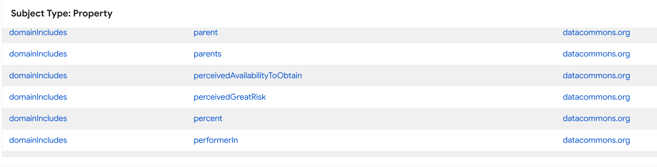

    

  • Use the Node API, filtering on domainIncludes incoming arcs: https://api.datacommons.org/v2/node?key=AIzaSyCTI4Xz-UW_G2Q2RfknhcfdAnTHq5X5XuI&nodes=POPULATION_TYPE&property=%3C-domainIncludes, e.g. https://api.datacommons.org/v2/node?key=AIzaSyCTI4Xz-UW_G2Q2RfknhcfdAnTHq5X5XuI&nodes=Person&property=%3C-domainIncludes.

Note that all fields that reference another node in the graph must be prefixed by dcid: or dcs:, which are interchangeable. You may wish to add an optional namespace, separated by a slash (/); for example, who/Adult_curr_cig_smokers. All fields that do not reference another node must be in quotation marks.

The following fields are optional:

• statType: By default this is dcid:measuredValue, which is simply a raw value of an observation. If your variable is a calculated value, such as an average, a minimum or maximum, you can use minValue, maxValue, meanValue, medianValue, sumvalue, varianceValue, marginOfError, stdErr. In this case, your data set should only include the observations that correspond to those calculated values.
• measurementQualifier: This is similar to the observationPeriod field for CSV observations (see below) but applies to all observations of the variable. It can be any string representing additional properties of the variable, e.g. Weekly, Monthly, Annual. For instance, if the measuredProperty is income, you can use Annual or Monthly to distinguish income over different periods. If the time interval affects the meaning of variable and and values change significantly by the time period, you should use this field keep them separate.
• measurementDenominator: For percentages or ratios, this refers to another statistical variable. For example, for per-capita, the measurementDenominator is Count_Person.

Additionally, you can specify any number of property-value pairs representing the constraints on the type identified by populationType. In our example, there is one constraint property, gender, which is a property of Person. The constraint property values are typically enumerations; such as genderType, which is a rangeIncludes property of gender. These will become additional sub-categories of the population type and displayed as such in the Statistical Variable Explorer. Using our example:

(Optional) Define a statistical variable group

If you would like to display variables in specific named groups, you can create a statistical variable group. You can actually define a hierarchical tree of categories this way.

Tip: If you are using implicit schema, where your variables are defined in the .csv files only (and optionally in config.json), and you want to assign variables to multiple groups, you can simply create an MCF file like the one below, and just specify the Node and memberOf fields for each variable.

Here is an example that defines a single group node with the heading “WHO” and assigns all 3 statistical variables to the same group.

Node: dcid:Adult_curr_cig_smokers
...
memberOf: dcid:who/g/WHO

Node: dcid:Adult_curr_cig_smokers_female
...
memberOf:dcid:who/g/WHO

Node: dcid:Adult_curr_cig_smokers_male
...
memberOf: dcid:who/g/WHO

Node: dcid:who/g/WHO
typeOf: dcid:StatVarGroup
name: "WHO"
specializationOf: dcid:dc/g/Root

You can define as many statistical variable group nodes as you like. Each must include the following fields:

• Node: This is the DCID of the group you are defining. It must be prefixed by g/ and may include an additional prefix before the g.
• typeOf: In the case of statistical variable group, this is always dcid:StatVarGroup.
• name: This is the name of the heading that will appear in the Statistical Variable Explorer.
• specializationOf: For a top-level group, this must be dcid:dc/g/Root, which is the root group in the statistical variable hierarchy in the Knowledge Graph.To create a sub-group, specify the DCID of another node you have already defined. For example, if you wanted to create a sub-group of WHO called Smoking, you would create a “Smoking” node with specializationOf: dcid:who/g/WHO. Here’s an example:

Node: dcid:who/g/WHO
typeOf: dcs:StatVarGroup
name: "WHO"
specializationOf: dcid:dc/g/Root

Node: dcid:who/g/Smoking
typeOf: dcs:StatVarGroup
name: "Smoking"
specializationOf: dcid:who/g/WHO

You can also assign a variable to as many group nodes as you like: simply specify a comma-separated list of group DCIDs in the memberOf. For example, to assign the 3 variables to both groups:

Node: dcid:Adult_curr_cig_smokers
...
memberOf: dcid:who/g/WHO, dcid:who/g/Smoking

Node: dcid:Adult_curr_cig_smokers_female
...
memberOf: dcid:who/g/WHO, dcid:who/g/Smoking

Node: dcid:Adult_curr_cig_smokers_male
...
memberOf: dcid:who/g/WHO, dcid:who/g/Smoking

Step 2: Prepare the CSV observation files

CSV files using explicit schema contain the following columns using the following headings:

entity, variable, date, value [, unit] [, scalingFactor] [, measurementMethod] [, observationPeriod]

The columns can be in any order, and you can specify custom names for the headings and use the columnMappings field in the JSON file to map them accordingly (see below for details).

These columns are required:

• entity: The DCID of an existing entity in the Data Commons knowledge graph, typically a place.
• variable: The DCID of the node you have defined in the MCF.
• date: The date of the observation and should be in the format YYYY, YYYY-MM, or YYYY-MM-DD.
• value: The value of the observation and must be numeric. The variable values must be numeric. Zeros and null values are accepted: zeros will be recorded and null values ignored.

Note: The type of the entities in a single file should be unique; do not mix multiple entity types in the same CSV file. For example, if you have observations for cities and counties, put all the city data in one CSV file and all the county data in another one.

The remaining columns are optional, and allow you to specify additional per-observation properties; see the descriptions of these in the JSON config file reference.

Here is an example of some real-world data from the WHO on the prevalance of smoking in adult populations, broken down by sex, in the correct CSV format:

SERIES,GEOGRAPHY,TIME_PERIOD,OBS_VALUE
dcs:who/Adult_curr_cig_smokers_female,dcid:country/AFG,2019,1.2
dcs:who/Adult_curr_cig_smokers_male,dcid:country/AFG,2019,13.4
dcs:who/Adult_curr_cig_smokers,dcid:country/AFG,2019,7.5
dcs:who/Adult_curr_cig_smokers_female,dcid:country/AGO,2016,1.8
dcs:who/Adult_curr_cig_smokers_male,dcid:country/AGO,2016,14.3
dcs:who/Adult_curr_cig_smokers_female,dcid:country/ALB,2018,4.5
dcs:who/Adult_curr_cig_smokers_male,dcid:country/ALB,2018,35.7
dcs:who/Adult_curr_cig_smokers_male,dcid:country/ARE,2018,11.1
dcs:who/Adult_curr_cig_smoking_female,dcid:country/ARE,2018,1.6
dcs:who/Adult_curr_cig_smokers,dcid:country/ARE,2018,6.3

In this case, the columns need to be mapped to the expected columns listed above; see below for details.

Step 3: Write the JSON config file

You must define a config.json in the top-level directory where your CSV files are located. With the explicit schema method, you need to provide these specifications:

• The input files location and entity type
• The sources and provenances of the data
• Column mappings, if you are using custom names for the column headings

Here is an example of how the config file would look for the CSV file we defined above. More details are below.

{
  "inputFiles": {
    "adult_cig_smoking.csv": {
      "provenance": "UN_WHO",
      "format": "variablePerRow",
      "columnMappings": {
        "variable": "SERIES",
        "entity": "GEOGRAPHY",
        "date": "TIME_PERIOD",
        "value": "OBS_VALUE"
      }
    }
  },
  "groupStatVarsByProperty": true,
  "sources": {
    "custom.who.int": {
      "url": "https://custom.who.int",
        "provenances": {
          "UN_WHO": "https://custom.who.int/data/gho/indicator-metadata-registry/imr-details/6128"
        }
    }
  }
}

The following fields are specific to the variable-per-row format:

• input_files:
  • format must be variablePerRow (the default is variablePerColumn if not specified)
  • columnMappings are required if you have used custom column heading names. The format is DEFAULT_NAME : CUSTOM_NAME.
• groupStatVarsByProperty is optional, and allows you to group your variables together according to population type. They will be displayed together in the Statistical Variable Explorer.

Note that you don’t specify your MCF files as input files; the Data Commons importer will identify them automatically.

The other fields are explained in the Data config file specification reference.

Load local custom data

The following procedures show you how to load and serve your custom data locally.

To load data in Google Cloud, see instead Load data in Google Cloud for procedures.

Configure environment variables

Edit the env.list file you created previously as follows:

• Set the INPUT_DIR variable to the full path to the directory where your input files are stored.
• Set the OUTPUT_DIR variable to the full path to the directory where you would like the output files to be stored. This can be the same or different from the input directory. When you rerun the Docker data management container, it will create a datacommons subdirectory under this directory.

Start the Docker containers with local custom data

Once you have configured everything, just run the run_cdc_dev_docker.sh script again. For reference, we provide the Docker commands invoked by the script below.

./run_cdc_dev_docker.sh

    docker run \
    --env-file $PWD/custom_dc/env.list \
    -v INPUT_DIRECTORY:INPUT_DIRECTORY \
    -v OUTPUT_DIRECTORY:OUTPUT_DIRECTORY \
    gcr.io/datcom-ci/datacommons-data:stable
    

    docker run -it \
    -p 8080:8080 \
    -e DEBUG=true \
    --env-file $PWD/custom_dc/env.list \
    -v INPUT_DIRECTORY:INPUT_DIRECTORY \
    -v OUTPUT_DIRECTORY:OUTPUT_DIRECTORY \
    gcr.io/datcom-ci/datacommons-services:stable
    

Note: Any time you make changes to the CSV or JSON files and want to reload the data, you need to restart both containers.

(Optional) Start the data management container in schema update mode

If you have tried to start a container, and have received a SQL check failed error, this indicates that a database schema update is needed. You need to restart the data management container, and you can specify an additional, optional, flag. This mode updates the database schema without re-importing data or re-building natural language embeddings. This is the quickest way to resolve a SQL check failed error during services container startup.

./run_cdc_dev_docker.sh --schema_update

    docker run \
    --env-file $PWD/custom_dc/env.list \
    -v INPUT_DIRECTORY:INPUT_DIRECTORY \
    -v OUTPUT_DIRECTORY:OUTPUT_DIRECTORY \
    -e DATA_RUN_MODE=schemaupdate
    gcr.io/datcom-ci/datacommons-data:stable
    

    docker run -it \
    -p 8080:8080 \
    -e DEBUG=true \
    --env-file $PWD/custom_dc/env.list \
    -v INPUT_DIRECTORY:INPUT_DIRECTORY \
    -v OUTPUT_DIRECTORY:OUTPUT_DIRECTORY \
    gcr.io/datcom-ci/datacommons-services:stable
    

Verify your data

If the servers have started up without errors, check to ensure that your data is showing up as expected.

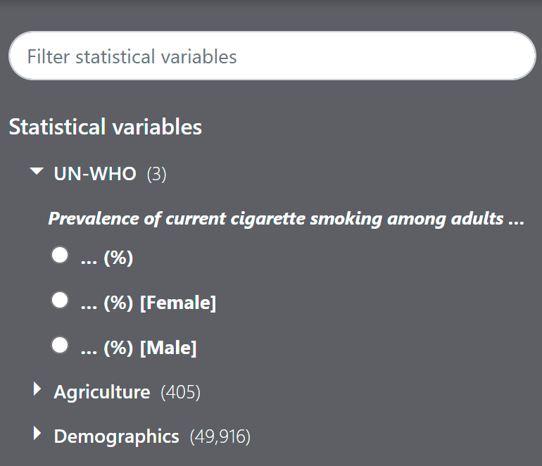
1. Verify statistical variables: go to the Statistical Variable Explorer to verify that your statistical variables are showing up correctly. You should see something like this:

   

2. Click on a variable name to get more information on the right panel.
3. Verify that your observations are loaded: Click on an Example Place link to open the detailed page for that place. Scroll to the bottom, where you should see a timeline graph of observations for the selected place.
4. Verify natural-language querying: go to the Search page and enter a query related to your data. You should get relevant graphs using your data.

Inspect the SQLite database

If you need to troubleshoot custom data, it is helpful to inspect the contents of the generated SQLite database.

To do so, from a terminal window, open the database:

sqlite3 OUTPUT_DIRECTORY/datacommons/datacommons.db

This starts the interactive SQLite shell. To view a list of tables, at the prompt type .tables. The relevant table is observations.

At the prompt, enter SQL queries. For example, for the sample OECD data, this query:

sqlite> select * from observations limit 10;

returns output like this:

country/BEL|average_annual_wage|2000|54577.62735|c/p/1
country/BEL|average_annual_wage|2001|54743.96009|c/p/1
country/BEL|average_annual_wage|2002|56157.24355|c/p/1
country/BEL|average_annual_wage|2003|56491.99591|c/p/1
country/BEL|average_annual_wage|2004|56195.68432|c/p/1
country/BEL|average_annual_wage|2005|55662.21541|c/p/1
...

To exit the sqlite shell, press Ctrl-D.

Page last updated: May 27, 2025 • Send feedback about this page